")
Today’s article is the fourth installment in the Trend Composite series. We started with an introduction to the Trend Composite, tested uptrend/downtrend signals and then moved to portfolio level testing using StochClose as the tiebreak. Today we focus more on StochClose rank by using it to select among ETFs where the Trend Composite is already positive (uptrend). The first test will use all 97 ETFs and I will then separate the bear market ETFs.
Trend Composite Strategy Series
- Introduction to the Trend Composite and its Indicators (1-Feb)
- Trend Composite Signal and StochClose Ranking Table (2-Feb)
- All Signals Tests and Indicator Comparison (8-Feb)
- Trend Portfolio: TrendComp Crosses, StochClose Rank, Mkt Regime (15-Feb)
- Momentum Portfolio: Trend Status, StochClose Rank, Bear Mkt ETFs (22-Feb)
- The All Weather Portfolio, Bull-Bear Market ETFs, Market Regime (17-Mar)
- Adding an ATR Trailing Stop and Time Based Exits (24-Mar)
- Live Example when Market Regime Turns Bullish (28-Mar).
- Adding a Percent Based Profit Target (31-Mar)
Note that the Trend Composite is part of the TIP Indicator Edge Plugin for StockCharts ACP. I use Amibroker because this is where I can build the indicators, test the indicators and fully customize the chart views.
The charts are linked to a SharpChart with corresponding indicators or the SharpChart alternatives. Note that CCI is used instead of CCI Close, Full Stochastic (125,5,1) is used instead of StochClose (125,5) and the thick black line is the 125-day SMA.
StochClose as a Ranking Mechanism
The strategy in this article buys ETFs with a positive Trend Composite value and the highest StochClose values. This means buying ETFs that are in uptrends and leading.
StochClose is used for ranking because it provides a volatility-adjusted score for price strength over the last six months (125 days). Keep in mind that 125-day StochClose measures the position of price relative to the 125-day high-low range. Values above 90 indicate that price is near a six month high, values below 10 indicate that price is near a six month low and values around 50 indicate that price is in the middle of its six month range.

Performance ranking is nothing new to trend-momentum strategies. The most popular momentum rank is probably Rate-of-Change (ROC), which is the percentage change over a given time period. There is nothing wrong with using Rate-of-Change to catch the high-flyers, but ROC rewards volatility and penalizes mundane ETFs.
Consider the Technology SPDR (XLK) and the Consumer Staples SPDR (XLP). XLK is the high-flyer with higher volatility, while XLP is more mundane with lower volatility. XLP is rarely going to win a Rate-of-Change contest against XLK, but it has a fighting chance with StochClose.
The charts below show the 125-day Rate-of-Change and StochClose (125,5) for comparison over the last two and a half years. ROC(125) regularly exceeded 20% for XLK, but only gets above 20% for a few weeks with XLP. StochClose, on the other hand, is regularly above 70 for both and reaches 100 several times for both.


StochClose levels the playing field and this increases the chances for diversification by opening the door for ETFs with lower volatility and strong uptrends. The 20+ Yr Treasury Bond ETF (TLT), DB Agriculture ETF (DBA), Utilities SPDR (XLU) and Consumer Staples SPDR (XLP) have relatively low volatility, but I do not want to exclude them from a trading strategy. Diversification spreads the risk and makes for a more balanced portfolio.
ETF Universe
The testing will cover 97 ETFs that have trading history back to at least 2007.
14 Non Equity ETFs
AGG, DBA, DBB, DBC, DBE, GLD, IEF, IEI, LQD, MBB, MUB, SLV, TIP, TLT
83 Equity-Related ETFs (includes 2 junk bond ETFs)
CGW, CUT, DIA, FCG, FDN, GDX, HYG, IBB, IGE, IGN, IGV, IHF, IHI, IJJ, IJK, IJR, IJS, IJT, ITA, ITB, IVE, IVW, IWC, IWD, IWF, IWM, IWN, IWO, IYR, IYT, IYZ, JNK, KBE, KIE, KRE, MDY, MOO, PBD, PBJ, PBW, PFF, PHO, PPA, PSP, QCLN, QQQ, RCD, REM, REZ, RGI, RHS, RSP, RTM, RYE, RYF, RYH, RYT, RYU, SDY, SHY, SLX, SOXX, SPHQ, SPIP, SPY, SUSA, VIG, XBI, XES, XHB, XLB, XLE, XLF, XLI, XLK, XLP, XLU, XLV, XLY, XME, XOP, XRT, XSD
Strategy Parameters
- Test period: 1/1/2007 to 1/31/2022 (15 years)
- 97 US ETFs with trading history back to at least 2007
- 14 Equal-weight Positions
- Buy/Sell based on opening prices the next day
- Commission: $5 per trade (buy/sell = two trades)
- Slippage: 2.5 bps or .0025 percent per trade
- No dividends (article explaining why)
Key Performance Metrics
The Gain/Loss Ratio is the Average Gain divided by the Average Loss. This one is pretty straight forward. Trend-followers would like to see this ratio above 3.
Profit Factor equals the number of winners multiplied by Average Gain divided by the number of losers multiplied by the Average Loss. A Profit Factor of 2 means total profits are outpacing total losses by a two to one margin.
Expectancy, which is similar to Profit Factor, is a performance metric based on the Win Rate, Average Gain and Average Loss. If the Win Rate is below 50%, then the Average Gain needs to be higher than the Average Loss to generate positive expectancy. Strategies with low Win Rates, say 30%, need an Average Gain that is much larger than the Average Loss to offset the high Loss Rate, which is 70% when the Win Rate is 30%.
Trend-Momentum with and without Market Regime
The basic strategy is to buy ETFs in uptrends and narrow the list with a performance metric. First take ETFs with positive Trend Composite values (uptrends), rank these by StochClose (performance metric), and then buy the top 14. Sell when the Trend Composite turns negative. For the replacement, sort ETFs with positive Trend Composite values by StochClose and select the highest ranking ETF. Rinse and repeat. The image below comes from the ETF Trend Signals and Ranking Table.

Now for performance results. The first line on the table below shows results without a Market Regime filter. The Market Regime and stock market are bullish when the Composite Breadth Model (here) is positive and bearish when negative. 83 of the 97 ETFs are equity-related so that means lots of equity exposure in bear markets and the results show. The Compound Annual Return is just 4.7%, the Maximum Drawdown was 26.09%, the Win Rate was just 42% and the Profit Factor was 2.08. Not impressive.

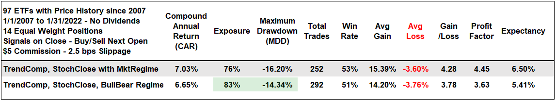
The second line shows results when using a Market Regime filter and we can see a big improvement right away. The Compound Annual Return hits 7%, the Maximum Drawdown is just 16.2%, the Win Rate exceeds 50% and the Profit Factor exceeds 4.
Do not underestimate the importance of the Market Regime when it comes to equity ETFs. Picking winners when the Market Regime is bearish is extremely difficult because correlations among equity groups rise in bear markets. This means buy or add new positions ONLY when the Market Regime is bullish. Do not buy and do not add new positions when the Market Regime is bearish. The normal sell signal applies for existing positions: sell when the Trend Composite turns negative.
Bull versus Bear Market ETFs
We can also consider dividing the ETF universe into two groups: All ETFs and Bear Market ETFs. All ETFs are eligible for trading during bull markets. Only bear market ETFs are eligible for trading during bear markets (Market Regime bearish). These are the non-equity ETFs: commodities, bonds and currencies.
The next table compares results when trading according to the Market Regime and dividing the ETF universe into two parts. The Compound Annual Return dipped to 6.65%, but the Maximum Drawdown also fell (14.4%) and this shows less risk. Exposure when up because this strategy was partially active during bear markets. The Win Rate, Gain/Loss Ratio, Profit Factor and Expectancy were not as good, but still respectable overall.
Note that the equity-related ETFs are not sold indiscriminately when the Market Regime turns bearish. They are sold when/if their Trend Composite turns negative (sell signal).
Perspective on Returns and Drawdowns
The next charts cover the last strategy, which divides the ETFs into two groups (All ETFs and Bear Market ETFs). The market surge from March 2020 until November 2021 was phenomenal and we should not get caught up in recency bias. These charts put overall performance into perspective by going back to 2007.
The first chart shows the equity curve for the strategy. Equity was flat in 2007 and 2008, even though the bear market ETFs were eligible for trading. There is a nice uptrend in this equity curve (green line) and this trend is punctuated with at least six sharp drawdowns (red shading). The most recent occurred in January 2022.

The next chart shows the strategy’s equity line (green line) outperforming SPY buy-and-hold until 2019. Buy-and-hold SPY (blue line) surged from mid 2020 until late 2021 as momentum stocks and ETFs led. Even though this bull-bear ETF strategy underperformed during this momentum period, I think this period was more of an exception than the new normal.

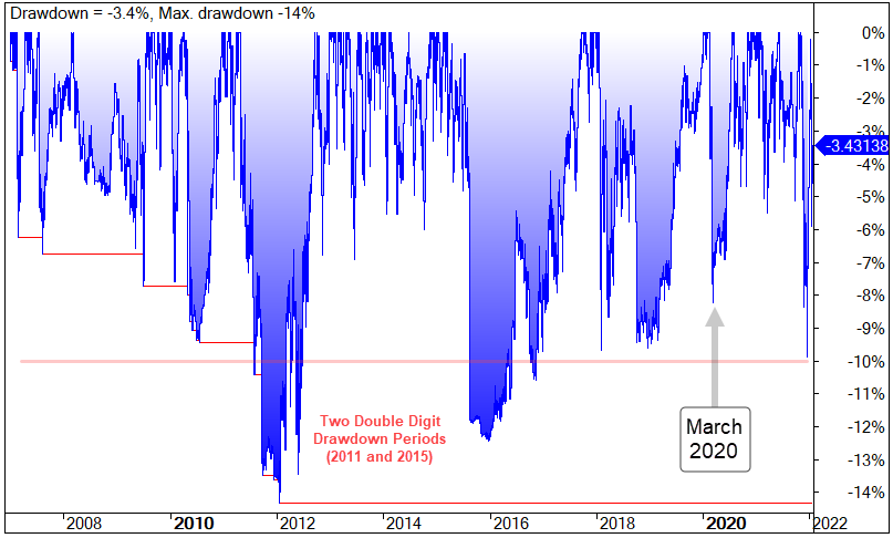
The next chart shows the drawdowns with two periods dipping below 10% (2011 and 2015). Even the drawdown in March 2020 held above the 10% level. Note that SPY experienced a 50% drawdown in 2008 and a 33% drawdown in March 2020.
The last table shows the monthly and yearly returns. There were three down years and twelve up years (not counting 2022). The biggest down year was 7.2% (2015) and the biggest up year was 24.9% (2013). Overall, monthly returns are quite mixed since June 2021 with four up months and four down months.

Conclusions
For 13 of the last 15 years, the bull-bear ETF strategy beat buy-and-hold SPY or performed inline with much better drawdowns. Even though momentum madness took over and led SPY to superior returns recently, the market goes through cycles and we could see a reversion to the mean (momentum lagging).
Investors can reduce drawdowns by insuring diversification, dampening momentum and using a Market Regime filter. We can insure diversification by having an ETF universe that includes non-equity ETFs and mundane ETFs. There is nothing wrong with high-beta and high-flying ETFs, but we need a universe that is in balance. Otherwise, the portfolio will be prone to some big swings.
StochClose can be used to dampen momentum and put ETFs on an equal footing when measuring price performance. And finally, trading according to the Market Regime can greatly reduce drawdowns because it cuts exposure to equity related ETFs during bear markets. Bear market ETFs can be used when the Market Regime is bearish.